A Beginner's Guide to Falling in Love with Algorithms - Part 2: Algorithm Design

With a backpack filled with the fundamentals of algorithmic complexity, we are ready to dive into the topic of this blogpost - algorithm design. Furthermore, using our newly acquired knowledge, we are able to analyze the computational tractability of these algorithms.

An algorithm that runs in polynomial time for an input size n is said to be tractable. If you are unfamiliar with polynomial time, I suggest you pause and read up on this before continuing. We categorize problems, which are solvable in polynomial time, as P problems. Conversely, an algorithm that runs in exponential time or worse for an input size n is said to be intractable. We categorize problems, for which we have not yet found a tractable polynomial time algorithm, as NP problems, i.e. non-polynomial meaning they are not solvable in polynomial time. We will not be covering NP problems in this particular series of posts.

Algorithm design consists of two parts, the design and analysis of an algorithm. In the design of the algorithm, we categorize the problem in accordance with the family of algorithms, for which the optimal algorithm for solving said problem is to be found. Then, by inspiration of algorithms from this family, we design an algorithm, which solves the problem at hand.

In the analysis of the algorithm, we start by determining the running time of the algorithm, with which we can determine the computational tractability of the algorithm, to quickly discard an intractable algorithm. Then, we determine the correctness of the algorithm, which is asserted by proving that it always produces the optimal and correct solution to the problem.

Let's see some examples of both the design and analysis of some algorithms. Through these examples, we will learn about three of said families of algorithms, albeit many more exist for you to discover.

Greedy Algorithms

An algorithm is known as greedy, if it builds up a solution in small steps, by choosing the locally optimal solution at each step, based on some criterion, towards a solution. Often, this success criterion is based on the structure of the problem, which we will see in the forthcoming example.

For the analysis of greedy algorithms, a common approach is to establish that the greedy algorithm stays ahead. In other words, at each step, one establishes that no other algorithm can do better, until it finally produces the optimal solution.

Interval Scheduling - Designing a Greedy Algorithm

For this algorithm, we will prove its correctness by establishing that the greedy algorithm stays ahead. Now let’s get into a problem, for which we will go through all the steps in the design of an algorithm that solves this problem. We start by presenting the problem:

We have a set of appointments, {1, 2,..., n}, where the i^th appointment corresponds to an interval spanning from a starting time, call it s_i, to a finishing time, call it f_i. We say that a subset of the intervals (a collection of said intervals) are compatible , if no two of the intervals overlap in time. Our goal is to accept as large a compatible subset as possible.

In other words, an optimal solution to our problem is one that always picks the largest number of appointments, for which none of them overlap in their starting and finishing time. Give the definition another glance, if you are not completely sure yet, which problem we are trying to solve.

Designing the algorithm

Finally, we are ready to design an algorithm. The process of doing so is often governed by the definition of a set of rules, which ultimately defines the algorithm. Therefore, it is often very helpful to start out by specifying and concretizing these, before getting into the specifics of the algorithm.

In our algorithm for interval scheduling, naturally, we need to start by selecting our first interval, call it i₁, and discarding all intervals, which are not compatible with said interval i₁ (remember our definition of compatible intervals). We then continue in this manner until we run out of intervals, which leaves us with a solution. This must mean that the optimality of said solution is governed by the rule, which we use to select said intervals. Great, so using our definition of the problem, we brainstorm ideas for a definition of a rule for selecting the "right" intervals, which will lead to the optimal solution.

An obvious contender for a rule, which comes to mind, is to select the interval that starts the earliest, i.e. the one with minimal starting time, s_i, which is still available, hereby using up intervals as soon as possible. This rule does not yield the optimal solution, and I encourage you to figure out why before moving on. In fact, I encourage you to do so at every step of our brainstorm.
We depict a counterexample, where the earliest interval spans multiple intervals and also has the latest finishing time, in which case more intervals could optimally be satisfied.

Another rule, which then comes to mind, is to select the smallest interval, i.e. where f_i - s_i is the smallest. Again, this rule does not yield the optimal solution. We depict a counterexample, where picking the smallest interval satisfies a suboptimal amount of intervals.

Before presenting the rule, which does yield the optimal solution, I encourage you to stop reading now, and to come up with other alternatives.
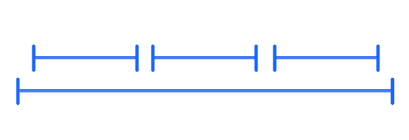
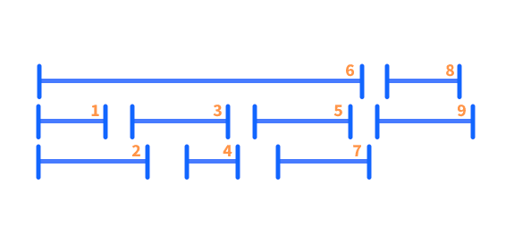
It turns out that the optimal solution in fact relies on the finishing time. Choosing the interval, which finishes first, i.e. the one with the minimal finishing time, f_i, will always yield the optimal solution. Intuitively, this makes sense, as we free up our resources as soon as possible. Again, I encourage you to convince yourself of the validity of this. If it helps you, you can use the below visualization for this approach.

With this in mind, we are ready to state our algorithm. We do so in pseudocode, which uses structural conventions common in most programming languages, but is otherwise a plain English description of the steps of the algorithm (Hint: Everything between the keywords While and EndWhile is repeated until the statement after the keyword While is true).

Let I be the set of all intervals.
Let A be the set of accepted intervals, which is initially empty
While I is not empty
    Choose interval i from I with the smallest finishing time
    Add interval i to A
    Remove all intervals not compatible with i from I
EndWhile
Return the set of all accepted intervals, A.

Analyzing the algorithm

In an analysis of an algorithm, one proves the correctness of the algorithm and determines the running time of said algorithm. We start with the proof of correctness.

First, by the steps of the algorithm, we can declare that the intervals of A are compatible, as we discard all non-compatible intervals, when we add an interval to A. Second, we must show that the solution is optimal, which is proven by induction. We will not get into the proof, but I will quickly describe the general idea. Let's consider theta, which represents an optimal solution, i.e. the set with the maximum amount of compatible intervals for a given collection of intervals. As many optimal solutions may exist, i.e. multiple combinations of compatible intervals, which would be of maximum size for a given collection, we should not prove that our solution A is equivalent to theta, i.e. A = theta. We should rather simply prove that the size of both sets are equal, i.e. |A| = |theta|. We do so by proving, that for all indices the following holds for the finishing times,

f(i_r) <= f(j_r)

where i_r and j_r are the r^th accepted intervals of A and theta, respectively. The proof by induction start by realizing that

f(i₁) <= f(j₁)

by the greedy rule of our algorithm, which states that we start by picking the interval with the earliest finishing time. That was quite a lot of theory and proofs of correctness.

We now move on to the running time. We can show, that our algorithm runs in time O(n log n), which we learned is linearithmic time in the previous blog post (part 1). Let us learn why this is the case by considering an implementation of said algorithm. This will get quite technical, but I merely want to give you an idea of the process.

We start by sorting all intervals by their finishing time, f_i, starting from the earliest, which takes O(n log n) time. Then, we construct an array S, which contains the value s_i of interval i at position S[i] in the array, which takes O(n) time.

Then, using our sorted list, we select intervals in order of increasing finishing time, f_i, which starts by choosing the first interval. Then, we iterate the intervals until reaching the first interval, call it j, where s_j >= f_i, i.e. which starts at or after the finishing time of the selected interval. We find the starting time of the iterated intervals using the array S. We continue iterating subsequent intervals, until no more intervals exist, where s_j >= f_i. This process takes O(n) time, which leaves us with a total running time of O(n log(n)) + O(n) + O(n) = O(n log(n)).

Dynamic Programming

In a way, this family of algorithms represents the opposition to greedy algorithms, as it entails exploring all possible solutions. In dynamic programming, we solve a problem by decomposing it into a set of smaller subproblems, and then incrementally composing the solutions to these into solutions to larger problems. Importantly, to avoid computing the result of the same subproblem multiple times, we store or memoize results in order to avoid these unnecessary computations. Note, that another technique called tabulation also exists, which will not be covered.

Before getting into dynamic programming, it is essential that we understand the concept of recursion, as dynamic programming is simply somewhat of an optimization of this using memoization.

Recursion means to define a problem in terms of itself, which in programming relates to the process of a function calling itself. In such a process, the solution to one or more base cases are defined, from which the solution to larger problems are recursively defined. This might seem as pure gibberish, but fear not, we will learn by example momentarily. It is important to note that an iterative approach to dynamic programming also exists, which will not be covered.

Fibonacci Sequence

Let’s define the Fibonacci sequence, which will serve as our example problem for a recursive algorithm:

A series of numbers, where each number is the sum of the two preceding numbers, i.e. 1, 1, 2, 3, 5, 8, 13, 21...

Based on this definition, we define a recursive algorithm for finding the n^th Fibonacci number.

def fib(n)
    if n == 1 or n == 2 # (1) base case
        return 1
    else 
        return fib(n - 2) + fib(n - 1) # (2) recursive step

In figure XX, we’ve build a tree, which represent the recursive function calls of the above algorithm, when looking for the 4^th Fibonacci number, i.e. fib(4). Using this tree, we’ll go through one of the branches of the recursive algorithm.

Initially, we call the function with n = 4, which means we go down the else-branch of our algorithm, in which we return the addition of the result of two new calls to the same function, i.e. our recursive step (step 2). To figure out the result of these two function calls, we look at each function call individually, which is represented by the second layer of our tree.

Let’s focus at the right side of the tree, represented by fib(3). We see the same behaviour, which results in a third layer. Looking at the two function calls in the third layer, we notice that both of these go down the if-branch of our algorithm, i.e. our base case for which we return 1.

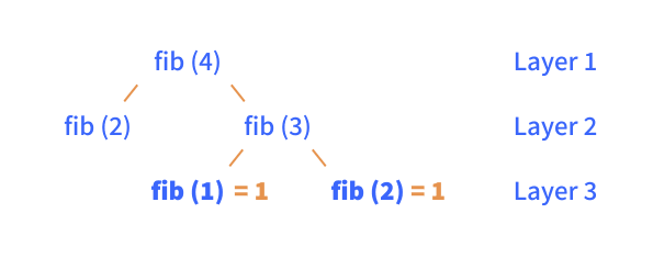
We now know the solution to fib(1) and fib(2), which we can return to the function call in layer 2. This in turn means that we return the solution to fib(3) = fib(1) + fib(2) = 2, i.e. the solutions to the smallest problems, at the bottom of the tree, cascade to the top, giving us the solution to our initial function call.

Designing the algorithm

If we look at the recursion tree of the previous implementation, we clearly see that the result of the same subproblem is calculated multiple times, which will results in an exponential-time algorithm. To exemplify the power of memoizing the result (caching), we will now see, how we can reduce a exponential-time algorithm, for finding the n^th Fibonacci number, to a linear-time one.

Now, instead of computing the same result multiple times, we design an algorithm, in which we memoize the result of previous subproblems, which we can then reuse. A dynamic programming algorithm is designed in three steps:

Define the subproblems in terms of the input.

Identify the base case(s).

Define the recursive step.

Let’s use these steps to define our algorithm. First, the subproblems comes naturally from the definition of the Fibonacci sequence, as the n^th Fibonacci number is based on the two preceding numbers.

Second, to make the Fibonacci sequence work, we need to define the first two numbers, as the n^th Fibonacci sequence is based on the two preceding numbers - we define fib(1) = 1 and fib(2) = 1.

Finally, based on the definition of our subproblems, our recursive step is defined by the decomposition of the n^th Fibonacci number, fib(n), i.e. fib(n) = fib(n - 2) + fib(n - 1), which we memoize to avoid computing the same result multiple times.

We now define our algorithm based on our initial design process:

cache = [] # (1) cache for memoization

def fib(n)      
    if n in cache:
        return cache[n] # (2) reuse old memoized/cached computation
    else:
        if n = 1 or n = 2: # (3) base case
            cache[n] = 1 # (4.1) memoize result
        else:
            cache[n] = fib(n - 2) + fib(n - 1) # (4.2) memoize result

    return cache[n]

Analyzing the algorithm

Using this approach, we never recompute any result in our recursion tree, but simply reuse the memoized result from the cache (step 2). As we memoize any result, which is not present in the cache (step 4), we do O(n) computations, which intuitively gives us a linear-time algorithm.

Divide and Conquer

We move on to the final family of algorithms for this blogpost, which closely resembles those of dynamic programming with some key differences. Despite being a well-known term, divide and conquer algorithms can be quite tricky to grasp, as they are, like most dynamic programming algorithms, also based heavily on recursion.

The divide and conquer family comprises a set of algorithms, in which the input is divided up into smaller sets of subproblems, each subproblem is conquered or solved recursively, and finally the solutions are combined into an overall solution.

The distinction between dynamic programming and divide and conquer is very subtle, as dynamic programming can be seen as an extension of divide and conquer. Both approaches work by solving subproblems recursively and combining these into a solution.
Dynamic programming algorithms exhaustively check all possible solutions, but importantly only solve the same subproblem once. The solution to a subproblem can then be reused in other overlapping subproblems using memoization or tabulation - the extension of the divide and conquer technique.
Divide and conquer algorithms do not reuse the solution of subproblems in other subproblems, as the subproblems are independent given the initial non-overlapping division of the problem.

Mergesort

The most famous subfamily of divide and conquer algorithms is definitely the sorting algorithms. In our example, we will present the mergesort algorithm, in which we will focus on the design of the algorithm. The analysis of divide and conquer algorithms include recurrence relations, which is outside the scope of our analysis.

Designing the algorithm

We wish to design an algorithm, which sorts a list A. The design of divide and conquer algorithms consists of defining three steps:

Divide the problem into subproblems

Conquer each subproblem by solving them recursively

Combine the result of each subproblem into a final solution

First, we define our divide step. Given an index m, representing the middle of the list, we divide our list into two smaller, equal-sized sublists. Second, in our conquer step, we recursively call the mergesort algorithm for our two new sublists. Finally, we merge the two sublists. Let’s see an implementation of this algorithm, which we can use as a reference.

def mergesort(l):
    if len(l) == 1:
        return l # base case
    mid = len(l) // 2
    left = l[:mid] # divide
    right = l[mid:] # divide
    a, b = mergesort(left), mergesort(right) # conquer
    return merge(a, b) # combine

def merge(a, b): # combine function
    l = list()
    i, j = 0, 0
    while i < len(a) and j < len(b): # 1. still elements in both lists
        if a[i] < b[j]:
            l.append(a[i])
            i += 1
        else:
            l.append(b[j])
            j += 1

    while i < len(a): # 2. still elements in a
        l.append(a[i])
        i += 1
    while j < len(b): # 3. still elements in b
        l.append(b[j])
        j += 1

    return l

Just like in dynamic programming, we continue in a recursive manner, until we reach our base case. In mergesort our base case is a list of length one that we cannot divide any further.

As we hit the base case, our two recursive mergesort() functions (line 7, conquer step) can now return two sorted lists, as they contain only one element. We will call these two lists a and b. Then, we pass these two lists to our merge() function, to merge the two lists (line 8).

Let’s visualize this with an example. First we divide the list by calling the mergesort() algorithm recursively with the two halves of the list, until we reach our base case. We focus on the left branch, as the process is similar for both branches.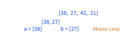

We’ve reached the base case for our recursion. Given our base case, in which the two lists contain only one element, we can now return two sorted lists to the previous recursive mergesort() function call, setting the two lists, a and b.

a, b = mergesort(left), mergesort(right)

Given these, we can call our merge() function, to sort the two lists (we will get into this function after the example).

We can now return this list to the recursive function above (or before) this function, which we will use to merge the list [27,38], with the sorted list from the other branch [21, 42], which eventually will give us our final merged, sorted list [21, 27, 38, 42].

In our merge step, we need to merge our two lists, which importantly are already sorted, into a combined, sorted list. We use two pointers, i for the list a and j for the list b, which helps us keep track of our progress in the two lists, in terms of adding elements to the new list.

In our merge step we proceed based on three different rules, which defines our algorithm, until all elements of lists a and b are present in the combined list.

If there are still elements left to be added from both lists, i.e. i < len(a) and j < len(b).

We check, which of the two elements at the index of our pointers are the smallest, and add that element to the combined list, as per this step of the merge function,

while i < len(a) and j < len(b): # 1. still elements in both lists
        if a[i] < b[j]:
            l.append(a[i])
            i += 1
        else:
            l.append(b[j])
            j += 1

Visualised as follows,

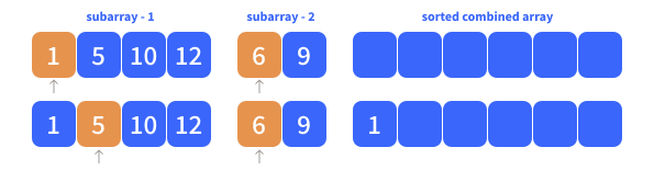
Where a[i] < b[j] is true, which is why we add 1 as the first element to the combined list.

If there are only elements left to be added for list a, in which case j < len(b) is no longer true, as j > len(b).

In this case we can simply add the remaining elements of list a to the combined list, as we know, that no element is smaller in b, given that b is empty.

while i < len(a): # 2. still elements in a
    l.append(a[i])
    i += 1

This is visualised as follows,

In which case we can simply add the elements 10 and 12 to the combined list.

If there are only elements left to be added for list b, in which case i < len(a) is no longer true, as i > len(a).

The process is equivalent to the latter, which is represented with the following code.

while j < len(b): # 3. still elements in b
    l.append(b[j])
    j += 1

When none of these three rules apply, our combined list is complete, and we can return it.

Analyzing the algorithm

We will not get into much detail in this analysis, but simply realize why this is a linearithmic algorithm, and why it is superior to the most intuitive way of sorting a set of numbers. Let’s look at an example of this for comparison.

Most people actually use an algorithm called selection sort, when they are to sort a set of playing cards. Given an list of numbers, a, of size n, where each number represents the value of each card in your hand, the algorithm works as follows,

Iterate over the list a[1] to a[n], and for each element a[i],

Compare the element to its predecessors, i.e. elements in the range a[1] to a[i-1].
Move all elements greater than a[i] up one position, essentially moving them to the right of a[i].

We give an example of a step using this algorithm, where n = 8, i = 6, and a[i] = 5, for which two elements are to be moved, to correctly position the element a[i].

If we look at a couple of steps of this algorithm,

It is clear, that at each step, we compare the element a[i] with one more element, until we finally compare the algorithm with all but one element, i.e. n - 1 elements. This means, that in average, we compare each element with n/2 elements, which gives us a total of n * n/2 comparisons. In asymptotic time, this means O(n²) comparisons, i.e. a quadratic running time. From the first blog post, we know that this is not a favorable running time.

Let’s return to mergesort and realize why this is a linearithmic time algorithm, i.e. superior to an algorithm of quadratic time (recall using https://www.bigocheatsheet.com/).

First, recall that x in log₂(n) = x, represents the number of times we can half our input size. Therefore, we can conclude, that the divide step of our algorithm divides our list into n single-element lists in O(log(n)) time.

Second, we convince ourselves, that recombining the list in the merge step of our algorithm takes O(n) time. Now, recall that our mergesort algorithm simply iterates over the two lists to combine them. In the worst case, the two lists are of length n/2, in which case it takes a total of O(n) time to iterate and combine the two lists.

Now, as we divided the initial list a total of O(log(n)) times, we must recursively merge that many lists to reach the final, sorted list. Therefore, the overall running time must be O(n * log(n)). Again, this might not be very intuitive, but in reality, the process of the analysis should be the real takeaway here.

What's to come?

We are still missing a very important family of algorithms, which we briefly mentioned in the start of this blogpost - NP algorithms. These are however deemed outside the scope of this blogpost, as it is simply not possible to cover this subject in less than a full blog post - we will leave this for another blog post.

The next and final blog post will go into depth with a specific family of algorithms - randomized algorithms. However, the focus of the blog post will be based on differential privacy, which utilizes randomized algorithms, and my thesis about this topic. In differential privacy one attempts to publicly share information about a population, without compromising the privacy of the individuals of said population. Tune in for the third and final blog post of this series for more on this.

References

https://jeffe.cs.illinois.edu/teaching/algorithms/book/04-greedy.pdf

Algorithm Design, Kleinberg and Tardos