Tutorial: Graph Neural Networks for Social Networks Using PyTorch

1. Set your expectations of this tutorial

You can follow this tutorial if you would like to know about Graph Neural Networks (GNNs) through a practical example using PyTorch framework.
I am aiming, at the end of this step-by-step tutorial, that you will be able to:

Gain insights about what graph neural networks (GNNs) are and what type of problems they may solve.

Know how graph datasets, which are expected by GNNs, look like. We will download and explore a social network dataset collected from GitHub.

Construct graphs and visualize them using code.

Construct and train a simple GNN model for node classification task based on convolutional GNN using torch_geometric, the geometric deep learning extension library for PyTorch.

Of course you are so welcome to post comments if you have any question or you feel that I deviated from what I promised you here!

2. GNN

\approx

Graph + Convolution Neural Network!

A BIG caveat here is to emphasize that I do not mean GNNs are just CNNs that operate on graphs, but what I want to say is that I felt comfortable with GNNs when I linked it to my understanding of CNNs and learnt something about graphs. For sure there are many other variations of GNNs but let us stick to this for those 10 minutes of reading. I hope this works for you as well, note that I put the $\approx$ sign to avoid causing some people to cringe.

Graph neural networks, as their name tells, are neural networks that work on graphs. And the graph is a data structure that has two main ingredients: nodes (a.k.a. vertices) which are connected by the second ingredient: edges. You can conceptualize the nodes as the graph entities or objects and the edges are any kind of relation that those nodes may have. Also you should know that both nodes and edges can have features (a.k.a. attributes), note the can as having features is not a must.

Mathematicians like to be concise and they represent the graph as the set

\mathcal{G = (V, E)}

where

\mathcal{G, V, E}

are the graph, vertices and edges sets respectively. But for our tutorial, let us make some visually appealing illustrations. The figure below represents a graph that consists of 4 nodes, represented by those blue circles with indices (1,2,3 and 4) and connected by directed edges represented by those green arrows. This graph is directed because the edges may represent asymmetric relationship, for instance if the nodes represent social network users and node 1 follows node 2 it does not mean that node 2 follows node 1. The contrary is the undirected graph which has bidirectional edges, then the relation could be friendship for example.

Since you are now reading this post about GNNs, I can confidently assume that you already have knowledge about CNNs. Yes, convolutional neural networks, the deep neural network class, that is most commonly applied to image analysis and computer vision applications.

Most of us, if not all, already know that images consist of pixels and the CNN leverages the convolution operation to calculate latent (hidden) features for different pixels based on their surrounding pixel values. It does this by sliding a kernel (a.k.a. filter) over the input image and calculating the dot product between that small filter and the overlapping image area. This dot product leads to aggregate the neighboring pixel values to one representative scaler. Now let us twist our conceptualization of images a little bit and think of images as a graphs. You can think of the pixels of the image as the nodes of the graph and the edges are present only between the adjacent pixels. You might have your own way to represent the image as a graph, what matters is that you just have the image-to-graph concept in your mind. If you get this then it is easier for you to think of GNNs as a generic version of CNNs that can operate on graphs.

The benefit of using GNNs is the provision of a generalized form that enables us to exploit non-Euclidean space data. In contrast to the pixels representation of images, the graph can be visualized as a collection of nodes and edges without having any order. So if we can learn node features in the latent space, we can do many interesting things. Those things are under three main categories:

Graph classification: where we can answer questions like: can we predict chemical compounds activity against lung cancer? Remember that chemical compounds can be represented as graphs with compound atoms as its nodes and chemical bonds are its edges.

Edge classification: as an example we can predict the congestion in a particular street, if we are given the city map. Then our graph has the streets as its edges and their intersections as its nodes.

Node classification: our tutorial problem falls under this category, as we are given a graph of a social network where users represent its nodes and the relationships between them are its edges and our task is to predict each user group (i.e. node class).

3. Adjacency matrix? Degree matrix? an example

Let us take a simple type of graphs, the undirected graph, this graph type is simple because the relationship between nodes is symmetric. Let us have an example of undirected graphs which has some numerical features attached to its nodes as well as its edges. Those features can represent any attributes that describe a node (blue boxes) or an edge (green boxes). Features are normally vectors, but we represent them by scalers here for simplicity.

We can express the above graph using two matrices which can capture its structure. The first is called the adjacency matrix and mostly denoted by A which is a square matrix used to represent finite graphs like this one. The elements of A indicate whether pairs of nodes are adjacent (i.e. connected by edges) or not in the graph. Those elements can be weighted (e.g. by edge features) as in our case; or can be unweighted (i.e. zeros
for disconnected nodes and ones for the adjacent nodes). For our graph we come up with a symmetric matrix with zero diagonal as shown below. The other matrix is the features matrix H (a.k.a. graph signal X) which holds the nodes' features of the graph.

An interesting operation that we may like to do is to calculate the dot product between those two matrices. This product, if we closely look at it, is generating a new feature vector that captures the feature of the surrounding nodes for each node based on how those surrounding nodes are connected to it. You can take a few seconds to relate the numbers on the calculation to the graph.

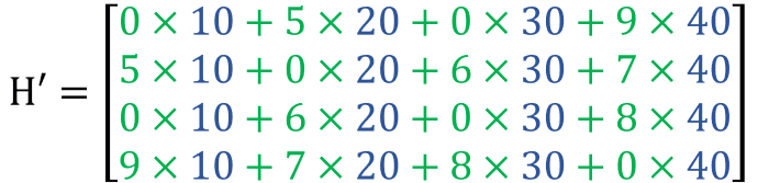
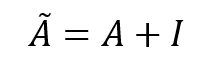
Now, if we take a critical look at the result we can observe two problems. The first is that when calculating the entry of the features matrix H' for any of the nodes we exclude that particular node features from the calculation as shown by red zeros. Which seems to be absurd! in the sense that we are ignoring our central node! To solve this we can add self-connections to every node on the graph and this can be achieved by adding the identity matrix ${I}$ to the graph adjacency matrix, which will alter its zero-valued diagonal to ones. So, now we can define the modified adjacency matrix $\tilde{A}$ as follows:

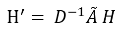
The second problem is the risk that may result from aggregating the features as we might end up with extremely high values which can lead to computation instability. We can see already signs of that in our simple example on the latent feature matrix H' which has entries at least 10 times more than the entries in the original H. The solution of this problem is to normalize the latent features by dividing by the graph degree matrix D (specifically we multiply by its inverse). The degree matrix is a diagonal matrix that contains information about the number of edges attached to each vertex. Our graph degree matrix looks like this:

Then the latent space feature representation can be calculated by the following, note that you may see different ways to solve this problem in the literature, but their common goal is to achieve some level of normalization by exploiting the graph structure:

4. Let us add some intelligence (learning)

So far, we discussed how we can calculate latent features of a graph data structure. But if we want to accomplish a particular task we can guide this calculation toward our goal. Particularly, we can leverage our last equation to be multiplied by a learnable weight matrix W and apply a nonlinear function to the product as in the next equation. We can learn the optimal W based on the task at hand. And here is where we can start doing interesting things.

Implementation wise, W can be a linear transformation (e.g. a linear layer) of the product and

\phi

is a non-linear activation function. I do not know if now you got the same intuition of mine (which is true) that we can stack as many functions of those as we like and learn the weight matrices W using backpropagation. Stacking those functions together promote this equation to be a deep learning model.

5. Time to get hands dirty!

Even though the above functions look natural and manageable to implement using many machine learning frameworks, torch_geometric (PyTorch Geometric), a geometric deep learning extension library for PyTorch, provides many variations of deep learning on graphs and other irregular structures.

Of course, as this field is evolving, you will find many interesting original GNN models and many "bells and whistles" for better suiting your problem. But for the sake of this tutorial, we will keep it simple and use only one flavor of GNNs which is the graph convolutional operator class GCNConv which is implemented from the paper “Semi-supervised Classification with Graph Convolutional Networks”, if you would like to have a look at how it was developed.

The particular problem we will be working on is a typical node classification problem. We have a large social network of GitHub developers named musae-github which was collected from the public API. Nodes represent developers (platform users) who have starred at least 10 repositories and edges are mutual follower relationships between them (note that word mutual indicates undirected relationship). The node features are extracted based on the location, repositories starred, employer and e-mail address. Our task is to predict whether the GitHub user is a web or a machine learning developer. This target feature was derived from the job title of each user. The dataset referenced paper is "Multi-scale Attributed Node Embedding".

Working with data, a golden rule is to learn as we go about the dataset. I am pasting here a dataset statistics table from the same source, so we can have a preliminary idea about what we are dealing with. This statistics tell us that our data set has those many nodes and those many edges. It also tells us that the edges has no features and no directions. Also, the data has no temporal property. All this information can give us a feeling that our dataset is a right candidate for this tutorial in term of simplicity.

After downloading the dataset, we can see 3 important files:
musae_git_edges.csv which contains the edges' indices.
musae_git_features.json which contains the nodes' features.
musae_git_target.csv which contains the targets, i.e. node labels.

5.1 Required packages

To begin with, we must download and import the required packages. To download torch_geometric please follow strictly the installation guide here, there are different options if you want to install using Pip Wheels, please check your syntax to download the compatible version based on your machine and software.
We will also need NetworkX Python package, we will use it to visualize the graph, I installed with pip. From torch_geometric we need to import AddTrainValTestMask, this will help us to segregate the training and test sets later. We also need json,pandas and numpy and some other packages.

%matplotlib inline

import json
import collections
import numpy as np
import pandas as pd

import matplotlib
import matplotlib.pyplot as plt

import torch
import torch.nn as nn
import torch.nn.functional as F

from torch_geometric.data import Data
from torch_geometric.transforms import AddTrainValTestMask as masking
from torch_geometric.utils.convert import to_networkx
from torch_geometric.nn import GCNConv

import networkx as nx

5.2 Dataset exploration

I assume the dataset files are in a subfolder named data. We read them and plot the top 5 rows and the last 5 rows from the labels file. Even though we see 4 columns but only 2 columns concern us here: id of the node (i.e. user) and ml_target which is 1 if the user is a machine learning community user and 0 otherwise. Now, we are sure that our task is a binary classification problem, as we only have 2 classes.

with open("data/musae_git_features.json") as json_data:
    data_raw = json.load(json_data)
edges=pd.read_csv("data/musae_git_edges.csv")
target_df=pd.read_csv("data/musae_git_target.csv")

print("5 top nodes labels")
print(target_df.head(5).to_markdown())
print()
print("5 last nodes")
print(target_df.tail(5).to_markdown())

Another important property we need to look at the class balance, this is because severe class imbalances may cause the classifier to simply guessing the majority class and not making any evaluation on the underrepresented class. By plotting the histogram (frequency distribution), we see some imbalance as the machine learning (label=1) are fewer than the other classes. This leads to some issues, but let us say, for now, it is not a severe problem.

We may also see how nodes are different based on the number of features. The second histogram tells that most of the users have between 15 and about 23 features, and very few of them have more than 30 and less than 5 features. The third histogram shows the most common features accross users, we can see different peaks on the distribution.

plt.hist(target_df.ml_target,bins=4);
plt.title("Classes distribution")
plt.show()

plt.hist(feat_counts,bins=20)
plt.title("Number of features per graph distribution")
plt.show()

plt.hist(feats,bins=50)
plt.title("Features distribution")
plt.show()

5.3 Features encoding

The nodes features tell us which feature is attached to each node. We can one-hot encode those features by writing our function encode_data. Our plan is to use this function to encode a light subset of the graph (e.g. only 60 nodes) for the purpose of visualization. Here is the function.

def encode_data(light=False,n=60):
    if light==True:
        nodes_included=n
    elif light==False:
        nodes_included=len(data_raw)

    data_encoded={}
    for i in range(nodes_included):# 
        one_hot_feat=np.array([0]*(max(feats)+1))
        this_feat=data_raw[str(i)]
        one_hot_feat[this_feat]=1
        data_encoded[str(i)]=list(one_hot_feat)

    if light==True:
        sparse_feat_matrix=np.zeros((1,max(feats)+1))
        for j in range(nodes_included):
            temp=np.array(data_encoded[str(j)]).reshape(1,-1)
            sparse_feat_matrix=np.concatenate((sparse_feat_matrix,temp),axis=0)
        sparse_feat_matrix=sparse_feat_matrix[1:,:]
        return(data_encoded,sparse_feat_matrix)
    elif light==False:
        return(data_encoded, None)

We can plot the first 250 features columns (the total is 4005) of the code for the first 60 users. Below, we can see how sparse is the matrix that we construct for nodes features.

data_encoded_vis,sparse_feat_matrix_vis=encode_data(light=True,n=60)
plt.figure(figsize=(25,25));
plt.imshow(sparse_feat_matrix_vis[:,:250],cmap='Greys');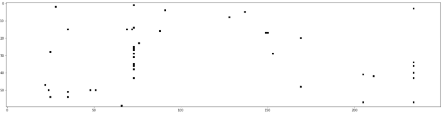

5.4 Graph construction and visualization

To construct our graph, we will use torch_geometric.data.Data which is a plain old python object to model a single graph with various (optional) attributes. We will construct our graph object using this class and passing the following attributes, noting that all arguments are torch tensors.

x: will be assigned to the encoded node features, its shape is [number_of_nodes, number_of_features].

y: will be assigned to the node labels, its shape is [number_of_nodes]

edge_index: to represent an undirected graph, we need to extend the original edge indices in a way that we can have two separate directed edges connecting the same two nodes but pointing opposite to each other. For example, we need to have 2 edges between node 100 and node 200, one edge points from 100 to 200 and the other points from 200 to 100. This is a way to represent the undirected graph if we are given the edge indecies. The tensor shape will be [2,2*number_of_original_edges].

It deserve mentioning here that this Data class is very abstract in a sense that you can add any attribute that you think it describes your graph. For instance we can add a metadata attribute g["meta_data"]="bla bla bla" which make it flexible to encapsulate any information you would like. Now, we will build construct_graph function which does the following:

def construct_graph(data_encoded,light=False):
    node_features_list=list(data_encoded.values())
    node_features=torch.tensor(node_features_list)
    node_labels=torch.tensor(target_df['ml_target'].values)
    edges_list=edges.values.tolist()
    edge_index01=torch.tensor(edges_list, dtype = torch.long).T
    edge_index02=torch.zeros(edge_index01.shape, dtype = torch.long)#.T
    edge_index02[0,:]=edge_index01[1,:]
    edge_index02[1,:]=edge_index01[0,:]
    edge_index0=torch.cat((edge_index01,edge_index02),axis=1)
    g = Data(x=node_features, y=node_labels, edge_index=edge_index0)
    g_light = Data(x=node_features[:,0:2],
                     y=node_labels   ,
                     edge_index=edge_index0[:,:55])
    if light:
        return(g_light)
    else:
        return(g)

For drawing a graph, we construct our draw_graph function. We need to convert our homogeneous graph to a NetworkX graph then pot using NetworkX.draw.

def draw_graph(data0):
    #node_labels=data0.y
    if data0.num_nodes>100:
        print("This is a big graph, can not plot...")
        return

    else:
        data_nx = to_networkx(data0)
        node_colors=data0.y[list(data_nx.nodes)]
        pos= nx.spring_layout(data_nx,scale =1)
        plt.figure(figsize=(12,8))
        nx.draw(data_nx, pos,  cmap=plt.get_cmap('Set1'),
                node_color =node_colors,node_size=600,connectionstyle="angle3",
                width =1, with_labels = False, edge_color = 'k', arrowstyle = "-")

Now, we can draw a sub graph by calling construct_graph with light=True. Then we can pass it to draw_graph, to show the following graph. You can see how the nodes are connected by edges and labeled by color.

g_sample=construct_graph(data_encoded=data_encoded_vis,light=True)
draw_graph(g_sample)

5.5 Construct and train our GNN model

We start by encoding the whole data by calling encode_data with light=False and construct the full graph by calling construct_graph with light=False. We will not try to visualize this big graph as I am assuming that you are using your local computer with limited resources.

data_encoded,_=encode_data(light=False)
g=construct_graph(data_encoded=data_encoded,light=False)

The usual immediate step after data preparation in the machine learning pipelines is to perform data segregation and split subsets of the dataset to train the model and further validate how it performs against new data and save a test segment to report the overall performance.

The splitting is not straight forward in our case as we have a single giant graph that should be taken all at once (there are some other ways to deal with graph segments, but let us assume this is the case for now). In order to tell the training phase which nodes that should be included during training and tell the inference phase which are the test data we can use masks which are binary vectors that indicate (using 0 and 1) which nodes belong to each particular mask. torch_geometric.transforms.AddTrainValTestMask class can take our graph and let us set how we want our masks to formed and it will add a node-level split via train_mask, val_mask and test_mask attributes. In our training, we use 30% as a validation set and 60% as test set while we keep only 10% for the training. You may have different split ratios, but in this way we may have a more realistic performance and we will not overfit easily (I know you might disagree with me on this point)! We can also print the graph information and the number of nodes each set (mask). The numbers between the brackets is the shape of each attribute tensor.

msk=masking(split="train_rest", num_splits = 1, num_val = 0.3, num_test= 0.6)
g=msk(g)
print(g)
print()
print("training samples",torch.sum(g.train_mask).item())
print("validation samples",torch.sum(g.val_mask ).item())
print("test samples",torch.sum(g.test_mask ).item())

At this point, I believe you agree with me that we are ready to construct our GNN model class. As we agreed we will use torch_geometric.nn.GCNConv class, however there are many other layers you can try on PyTorch Geometric documentation.
We will stack two GCNConv layers, the first has input features equal to the number of features in our graph and some arbitrary number of output features f. Then we apply a relu activation function and deliver the latent features to the second layer which has output nodes equal to the number our classes (i.e. 2). In the forward function, GCNConv can accept many arguments x as the nodes features, edge_index and edge_weight, in our case we only use the first two arguments.

class SocialGNN(torch.nn.Module):
    def __init__(self,num_of_feat,f):
        super(SocialGNN, self).__init__()
        self.conv1 = GCNConv(num_of_feat, f)
        self.conv2 = GCNConv(f, 2)

    def forward(self, data):
        x = data.x.float()
        edge_index =  data.edge_index
        x = self.conv1(x=x, edge_index=edge_index)
        x = F.relu(x)
        x = self.conv2(x, edge_index)
        return x

As our model will predict the class of all nodes in the graph, we, however, want to calculate the loss and accuracy for specific set based on the phase we are in. For instance, during training we want to calculate the training loss and accuracy only based on the training set and here where we should use our masks. We will define functions masked_loss and masked_accuracy for which we pass the respective masks and it returns the corresponding loss and accuracy. The idea is to calculate the loss and accuracy for all nodes and multiply it by the mask to zero out the not required nodes.

def masked_loss(predictions,labels,mask):
    mask=mask.float()
    mask=mask/torch.mean(mask)
    loss=criterion(predictions,labels)
    loss=loss*mask
    loss=torch.mean(loss)
    return (loss)    

def masked_accuracy(predictions,labels,mask):
    mask=mask.float()
    mask/=torch.mean(mask)
    accuracy=(torch.argmax(predictions,axis=1)==labels).long()
    accuracy=mask*accuracy
    accuracy=torch.mean(accuracy)
    return (accuracy)

Now, we can define our training function in which we will use torch.optim.Adam optimizer. We will run the training for some number of epochs and we keep track for the best validation accuracy. We also plot the losses and accuracies across epochs for the training.

def train_social(net,data,epochs=10,lr=0.01):
    optimizer = torch.optim.Adam(net.parameters(), lr=lr) # 00001
    best_accuracy=0.0

    train_losses=[]
    train_accuracies=[]

    val_losses=[]
    val_accuracies=[]

    test_losses=[]
    test_accuracies=[]

    for ep in range(epochs+1):
        optimizer.zero_grad()
        out=net(data)
        loss=masked_loss(predictions=out,
                         labels=data.y,
                         mask=data.train_mask)
        loss.backward()
        optimizer.step()
        train_losses+=[loss]
        train_accuracy=masked_accuracy(predictions=out,
                                       labels=data.y, 
                                       mask=data.train_mask)
        train_accuracies+=[train_accuracy]

        val_loss=masked_loss(predictions=out,
                             labels=data.y, 
                             mask=data.val_mask)
        val_losses+=[val_loss]

        val_accuracy=masked_accuracy(predictions=out,
                                     labels=data.y, 
                                     mask=data.val_mask)
        val_accuracies+=[val_accuracy]

        test_accuracy=masked_accuracy(predictions=out,
                                      labels=data.y, 
                                      mask=data.test_mask)
        test_accuracies+=[test_accuracy]
        if np.round(val_accuracy,4)> np.round(best_accuracy ,4):
            print("Epoch {}/{}, Train_Loss: {:.4f}, Train_Accuracy: {:.4f}, Val_Accuracy: {:.4f}, Test_Accuracy: {:.4f}"
                      .format(ep+1,epochs, loss.item(), train_accuracy, val_accuracy,  test_accuracy))
            best_accuracy=val_accuracy

    plt.plot(train_losses)  
    plt.plot(val_losses)
    plt.plot(test_losses)  
    plt.show()

    plt.plot(train_accuracies) 
    plt.plot(val_accuracies)
    plt.plot(test_accuracies) 
    plt.show()

At this point we constructed all the required functions and ready to instantiate our model and train it. We will construct the model with 16 filters and will use nn.CrossEntropyLoss as our loss criterion. Below, we can see that our simple model reached a very decent accuracy on the test set, more than 87%. We can also see the learning curves (losses) and accuracies development through epochs on the top and bottom plots respectively.

num_of_feat=g.num_node_features
net=SocialGNN(num_of_feat=num_of_feat,f=16)
criterion=nn.CrossEntropyLoss()
train_social(net,g,epochs=50,lr=0.1)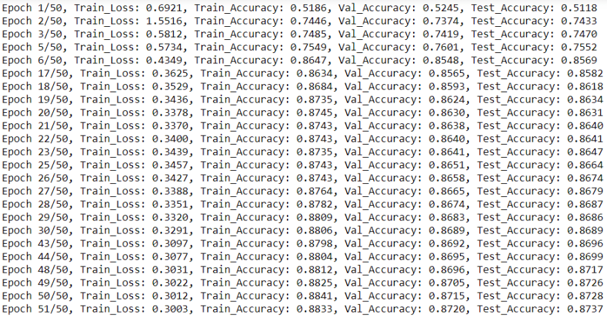

6. Conclusion and next steps

We have gone through this step-by-step tutorial covering fundamental concepts about graph neural networks and developed our simple GNN model based on convolutional GNN on PyTorch framework using torch_geometric extension. You might want to access the github repository of this code.