Achieving AI Prediction with e-RT3 Plus

A processed dataset for AI prediction must be available in .csv format. Here, we use the Iris dataset. However, any other dataset can be used in its place. The intention is to have valid data to enable prediction.

NOTE: The processed dataset file must not have any null, strings, objects, or any categorical data.

A sample AI application must be available for use.

NOTE: For more information about the Sample AI application, refer to Deploying a sample AI application on e-RT3 Plus.

Node-RED and modbus nodes must be installed on both e-RT3 Plus devices.

Modbus Slave Simulator, InfluxDB, and Grafana, must be installed on the server.

InfluxDB nodes must be installed on the prediction e-RT3 Plus.

Open an SSH terminal to the e-RT3 Plus device.

For more information about connecting to e-RT3 Plus using SSH, refer to Remote Communication with e-RT3 Plus.

Run the following command in the terminal to install the Modbus nodes.

cd /node_red
sudo npm install --force [email protected] [email protected]

The Modbus nodes are installed.

Download and install the Modbus Slave Simulator from the Modbus website.

Open Command Prompt.

Use the cd command to navigate to the directory where you installed the Modbus Slave Simulator.

Run the following command to start the Modbus/TCP server.

diagslave -m tcp 

Copy the sample Iris data set iris_data_target.csv to the following location in the simulator e-RT3 Plus by using WinSCP:

/home/ert3/datasets/

NOTE: You can upload your own dataset here instead of the Iris dataset.

For more information about how to use WinSCP for file transfer, refer to Using WinSCP to transfer files to e-RT3 Plus.

Specify the following URL in the address bar of your web browser:

{SIMULATOR_ERT3_IP_ADDRESS}:{NODE_RED_PORT_NUMBER}

NOTE: The default port number is 1880.

The Node-RED login page appears.

Log on to the editor by using your user credentials.

The Node-RED editor appears.

To inject data from the .csv file into the flow, perform these steps:

a. On the left pane, expand common, select the inject node, and drag it to the work area.

b. Double-click the created node.

The properties of the selected node are displayed on the right pane.

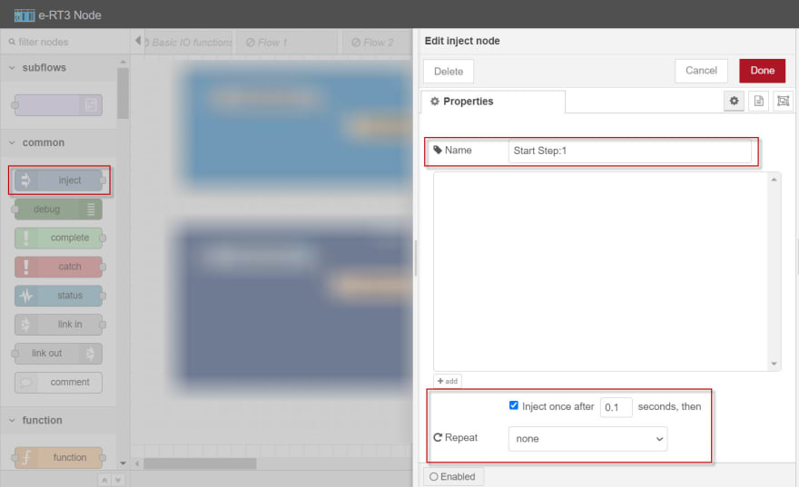
c. In the Name box, specify the name of the node.

d. Select the inject once after check box and specify the interval as 0.1 seconds for the data to be injected automatically.

e. From the Repeat drop-down list, select none.

f. In the upper-right corner of the page, click Done to save the changes.

To read the contents of the .csv file, perform these steps:

a. On the left pane, expand storage, select the file in node, and drag it to the work area.

b. Double-click the created node.

The properties of the selected node are displayed on the right pane.

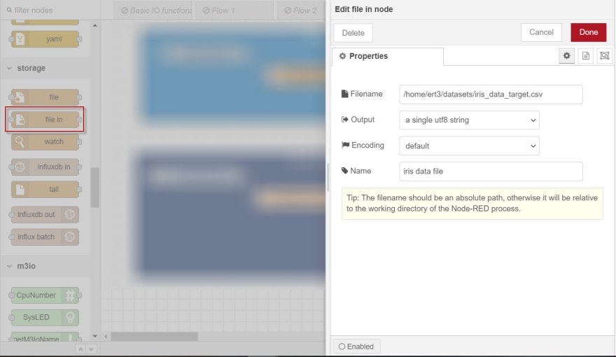
c. In the Filename box, specify the absolute path of the Iris dataset in the simulation e-RT3 Plus.

d. From the Output drop-down list, select a single utf8 string.

e. From the Encoding drop-down list, select default.

f. In the Name box, specify the name of the node.

g. In the upper-right corner of the page, click Done to save the changes.

To convert the csv data string into an object, perform these steps:

a. On the left pane, expand parser, select the csv node, and drag it to the work area.

b. Double-click the created node.

The properties of the selected node are displayed on the right pane.

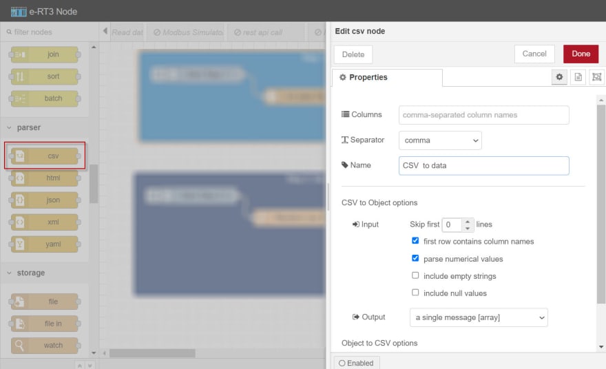
c. In the Name box, specify the name of the node.

d. From the Separator drop-down list, select comma.

e. Select the first row contains column names check box.

f. Select the parse numerical values check box.

g. From the Output drop-down list, select a single message [array].

h. In the upper-right corner of the page, click Done to save the changes.

To make the converted .csv data available for reading in the current flow context, perform these steps:

a. On the left pane, expand function, select the function node, and drag it to the work area.

b. Double-click the created node.

The properties of the selected node are displayed on the right pane.

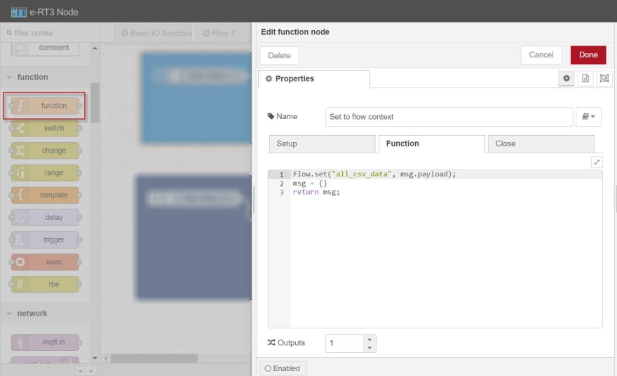
c. In the Name box, specify the name of the node.

d. Click the Function tab and type the following code in the editor.

flow.set("all_csv_data", msg.payload);
msg = {}
return msg;

e. In the upper-right corner of the page, click Done to save the changes.

Use connectors to connect all the nodes. The final flow should look something like this:

On the menu bar, click Deploy to activate the flow.

The data from the dataset is set to the flow context.

To inject data at a specified time interval, perform these steps:

a. On the left pane, expand common, select the inject node, and drag it to the work area.

b. Double-click the created node.

The properties of the selected node are displayed on the right pane.

c. In the Name box, specify the name of the node.

d. Select the inject once after check box and specify the interval as 10 seconds.

e. From the Repeat drop-down list, select interval and set the interval as 10 seconds.

f. In the upper-right corner of the page, click Done to save the changes.

To create a function that randomly selects a row of the Iris data, transforms it into an array and sends it to the Modbus Write node, perform these steps:

a. On the left pane, expand function, select the function node and drag it to the work area.

b. Double-click the created node.

The properties of the selected node are displayed on the right pane.

c. In the Name box, specify the name of the node.

d. Click the Function tab, and type the following code in the editor to create an array of the dataset, which will be sent to Modbus Write node.

const csvAsArray = flow.get("all_csv_data");
/* get random index value */
const randomIndex = Math.floor(Math.random() * csvAsArray.length);
/* get random item */
const item = csvAsArray[randomIndex];
const values = Object.keys(item || {}).map(function (key) {
    const value = item[key]
    return key == "Target"?value : Math.floor(value * 100);
});
msg = {
    topic: "Iris Dataset",
    payload: values
}
return msg;

NOTE: Since Modbus only accepts integers, the values are multiplied by 100 to convert float values to integers.

e. In the upper-right corner of the page, click Done to save the changes.

To write the data received at the node input to the Modbus Slave, perform these steps:

Note: This node is configured with the IP address of the Modbus Slave to indicate where the data must be sent. The address of the registers, as well as the size of data being sent, is specified in the node.

a. On the left pane, expand modbus, select the Modbus Write node, and drag it to the work area.

b. Double-click the created node.

The properties of the selected node are displayed on the right pane.

c. In the Name box, specify the name of the node.

d. From the FC drop-down list, select FC 16: Preset multiple Registers.

e. In the Address box, specify any address greater than zero.

f. In the Quantity box, specify 5 since the dataset has four independent variables and one target variable.

g. Next to the Server drop-down list, click the Edit icon and specify the following:

Type:   TCP
Host:   {SERVER_PC_IP_ADDRESS}
Port:   Specify the Modbus Slave Simulator port number. The default port number is 502.

h. Select the Show Errors check box.

i. In the upper-right corner of the page, click Done to save the changes.

To get the output message, on the left pane, select the debug node and drag it onto the work area twice. Use connectors to connect all the nodes. The final flow should look something like this:

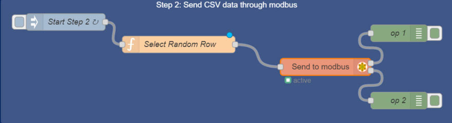
On the menu bar, click Deploy to activate the flow.

Data from the Iris dataset is transmitted to the Modbus Slave Simulator.

In the upper-right corner of the e-RT3 Node window, click the Debug tab.

Debug messages appear at an interval of 10 seconds in the Debug window.

Type the following URL in the address bar of your web browser:

{PREDICTION_ERT3_IP_ADDRESS}:{NODE_RED_PORT_NUMBER}

NOTE: The default port number is 1880.

The Node-RED login page appears.

Log on to the editor by using your user credentials.

The Node-RED editor appears.

To read the data that is being sent by the Modbus Slave, perform these steps:

Note: In this node, the IP address and the register details of the Modbus Slave are specified to identify the data source. The configured node will read the data sent by the Modbus Slave and forward it to the next node.

a. On the left pane, expand modbus, select the Modbus Read node, and drag it to the work area.

b. Double-click the created node.

The properties of the selected node are displayed on the right pane.

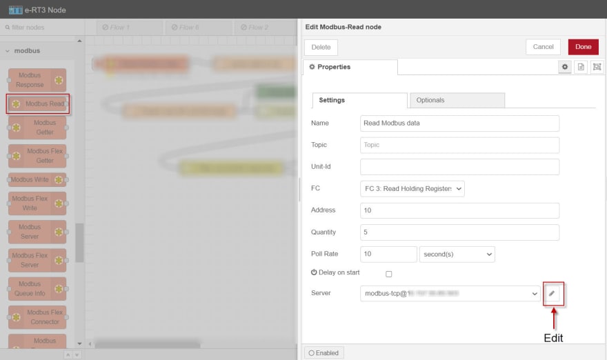
c. In the Name box, specify the name of the node.

d. From the FC drop-down list, select FC 3: Read Holding Registers.

e. In the Address box, specify the address given while creating the Modbus Write node in the previous flow.

f. In the Quantity box, specify 5 since the data being sent has four independent variables and one target variable.

g. In the Poll Rate box, specify the interval as 10 seconds.

h. Next to the Server drop-down list, click the edit icon and specify the following:

Type: TCP
Host: {SERVER_PC_IP_ADDRESS}
Port: Specify the Modbus Slave Simulator port number. The default port number is 502.

i. In the upper-right corner of the page, click Done to save the changes.

To format the data received at the node input for writing into InfluxDB, perform these steps:

a. On the left pane, expand function, select the function node, and drag it to the work area.

b. Double-click the created node.

The properties of the selected node are displayed on the right pane.

c. In the Name box, specify the name of the node.

d. Click the Function tab, and type the following code in the editor to get the array received by the simulator:

const dataArray = msg.payload

payload = {
    'Sepal_length': dataArray[0] / 100,
    'Sepal_width': dataArray[1] / 100,
    'Petal_length': dataArray[2] / 100,
    'Petal_width': dataArray[3] / 100,
}

msg["payload"] = payload
msg["data"] = { 
    'Actual_Target' : dataArray[4],
    'Features' : {...payload}
}
return msg;

NOTE: The values are divided by 100 to convert the integers back to float values.

e. In the upper-right corner of the page, click Done to save the changes.

To combine the features and the actual target sent by the previous node, into a single object to be written to InfluxDB. perform these steps:

a. On the left pane, expand function, select the function node, and drag it to the work area.

b. Double-click the created node.

The properties of the selected node are displayed on the right pane.

c. In the Name box, specify the name of the node.

d. Click the Function tab and type the following code in the editor:

const features = msg.data.Features
const target = msg.data.Actual_Target

const payload = {
    ...features,
    'target': target
}

msg["payload"] = payload

return msg;

e. In the upper-right corner of the page, click Done to save the changes.

To write the input data to the specified InfluxDB database, perform these steps:

a. On the left pane, expand storage, select the influxdb out node, and drag it to the work area.

b. Double-click the created node.

The properties of the selected node are displayed on the right pane.

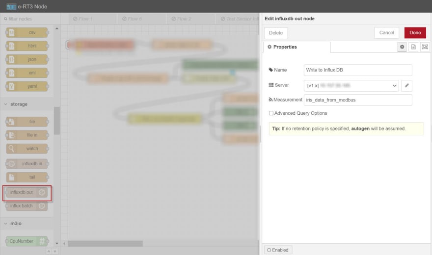
c. In the Name box, specify the name of the node.

d. Next to the Server drop-down list, click the edit icon and specify the following:

Version: TCP
Host: {SERVER_PC_IP_ADDRESS}
Port: The default port number is 8086.
Database: The name of the created InfluxDB database.
Measurement: Name of measurement. 

NOTE: The Name of measurement and Database name must be noted for future use. It will be used later to query data in Grafana and for exporting the data in InfluxDB to a .csv file.

e. In the upper-right corner of the page, click Update.

f. In the upper-right corner of the page, click Done to save the changes.

NOTE: For more information about how to create an InfluxDB database, refer to Create InfluxDB database.

Use connectors to connect all the nodes in the following manner.

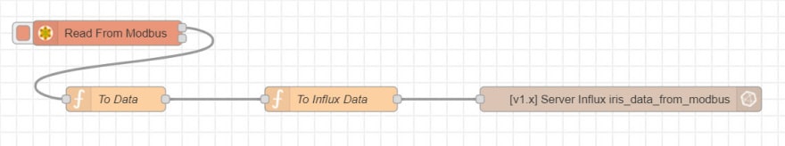
On the menu bar, click Deploy to activate the flow.

Run the following command to get the docker name.

docker ps 

A table appears, listing the active containers in Docker.

Locate the InfluxDB Docker container and run the following command to start communicating with InfluxDB.

docker exec -it {INFLUXDB_NAME} bash    

Here, {INFLUXDB_NAME} is the name of the InfluxDB container obtained from the previous step.

Run the following command to export the required data from InfluxDB to a .csv file.

influx -database "{CREATED_DB_NAME}" -execute 'SELECT * FROM "{REQUIRED_MEASUREMENT_NAME}"' -format 'csv' > /var/lib/influxdb/{CSV_FILE_NAME}.csv

Here, {CREATED_DB_NAME} refers to the name specified while creating the DB in InfluxDB, {REQUIRED_MEASUREMENT_NAME} refers to the name specified for the measurement while writing the data into the DB, and {CSV_FILE_NAME} refers to the name of the .csv file to be created.

Run the following command to exit the InfluxDB container.

exit

In the terminal, use the cd command to navigate to the folder where you want to store the .csv file.

Run the following command to copy the .csv file to the current folder.

docker cp {INFLUXDB_NAME}:/var/lib/influxdb/{CSV_FILE_NAME}.csv .

Remove all node connectors.

Note: The nodes will be reordered to modify the flow.

To package the data to be sent to the prediction algorithm, perform these steps:

Note: In this node, we configure the name of the data model to be used, and the values of the Iris dataset. This information is sent as a single object to the next node, which will call the prediction algorithm by using REST API.

a. On the left pane, select the function node, and drag it to the work area.

b. Double-click the created node.

The properties of the selected node are displayed on the right pane.

c. In the Name box, specify the name of the node.

d. Click the Function tab and type the following code in the editor to remove the Target value from the array before passing it to the prediction model.

const iris_data = msg.payload

const values = Object.keys(iris_data || {}).map(function (key) {
return key != "Target"?iris_data[key]:undefined;
});
msg["payload"] = {
    "model_name":"<name_of_the_generated_model>",
    "feature_values":values.filter(Boolean)
}    
return msg;

Note: The model name specified here is the model name that was generated while creating the data model in the Sample AI application.

e. In the upper-right corner of the page, click Done to save the pages.

To call the prediction algorithm is called using the REST API, perform these steps:

Note: This node sends a http request and returns the response.

a. On the left pane, expand network, select the http request node, and drag it to the work area.

b. Double-click the created node.

The properties of the selected node are displayed on the right pane.

c. From the Method drop-down list, select POST.

d. In the URL box, specify the following path of the REST API that is used for prediction:

http://{PREDICTION_ERT3_IP_ADDRESS}:9092/api/predictions  

e. From the Return drop-down list, select a parsed JSON object.

f. In the Name box, specify the name of the node.

g. In the upper-right corner of the page, click Done to save the changes.

To checks whether the prediction call is successful, perform these steps:

a. On the left pane, expand function, select the switch node, and drag it to the work area.

b. Double-click the created node.

The properties of the selected node are displayed on the right pane.

c. In the Name box, specify the name of the node.

d. In the Property box, select msg from the drop-down list and specify statusCode in the adjacent box.

e. Click add, and specify the following to route the output to port 1 in the prediction failure case:

    != 200

f. Click add, and specify the following to route the output to port 2 in the prediction success case:

    == 200

g. From the drop-down list at the bottom of the page, select stopping after first match.

h. In the upper-right corner of the Properties page, click Done.

To convert the input data into a format that can be written into InfluxDB, perform these steps:

Note: This node must be connected to port 2 of the switch node output to handle the success case.

a. On the left pane, expand function, select the function node, and drag it to the work area.

b. Double-click the created node.

The properties of the selected node are displayed on the right pane.

c. In the Name box, specify the name of the node.

d. Click the Function tab and type the following code in the editor:

const predicted_target = msg.payload.predicted_target
const features_headers = msg.payload.features.headers
const features_values = msg.payload.features.values
const actual_target = msg.data.Actual_Target

let payload = {}
features_headers.forEach(function(val,index) {
payload = {...payload, ...{
[val.toLowerCase()]:features_values[index]
}}
})
payload = {...payload, ...{
"target":actual_target,
"predicted_target":predicted_target
}}

msg.payload = payload
return msg;

e. In the upper-right corner of the page, click Done to save the changes.

On the left pane, select the debug node and drag it onto the work area. Set the debug node to show msg.payload.

Now we have all the necessary nodes on the work area. Use connectors to connect all the nodes. The final flow should look something like this.

On the menu bar, click Deploy to activate the flow.

The prediction e-RT3 Plus starts processing the incoming live data and the predictions are written into InfluxDB.

In the upper-right corner of the e-RT3 Node window, click the Debug tab.

The debug pane appears, displaying the values written to InfluxDB.

Type the following URL in the address bar of your web browser:

{SERVER_PC_IP_ADDRESS}:{PORT_NUMBER}

The Grafana login page appears.

NOTE: The default port number is 3000.

Log on to Grafana by using your user credentials

The Grafana Home page appears.

From the navigation menu on the left, click the Settings icon, and select Configuration > Data Sources.

Connect Grafana to InfluxDB.

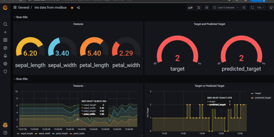
Add panels to the dashboard as necessary.

For more information on how to add and customize a panel, refer to Grafana website.

Configure your dashboard to suit your requirements.