
58
Logistic Regression
Welcome to the 3rd article of the Demystifying Machine Learning series. In this article, we are going to discuss a supervised classification algorithm Logistic Regression, how it works, why it's important, mathematics behind the scenes, linear and non-linear separation and Regularization.
A good grasp of Linear Regression is needed to understand this algorithm and luckily we already covered it, for reference you can read it from here. Logistic Regression builds the base of Neural Networks, so it gets very important to understand the terms and working of this algorithm.
Logistic Regression is not a regression algorithm, its name does consist of the word "Regression" but it's a classification algorithm.
Logistic Regression also known as Perceptron algorithm is a supervised classification algorithm i.e. we teach our hypothesis with categorical labelled data and it predicts the classes (or categories) with some certain probability. The reason this algorithm is called Logistic Regression is maybe that it's working is pretty similar to that of Linear Regression and the term "Logistic" is because we use a Logistic function in this algorithm (we'll going to see it later). The difference is that with Linear Regression we intend to predict the continuous values but with Logistic Regression we want to predict the categorical value. Like whether the student gets enrolled in a university or not, if the picture contains a cat or not, etc.
Here's a representation of how Logistic Regression classifies the data points.

We can see that the blue points are separated from the orange points through a line and we call this line a decision boundary. Basically, with Logistic Regression we separate the classes (or categories) with the help of decision boundaries, they can be linear or non-linear.
Let's revise what we learnt in Linear Regression, we initialise the parameters with all 0s, then with the help of Gradient Descent calculate the optimal parameters by reducing the cost function and lastly draw the hypothesis to predict the continuous-valued target.
But here we don't need continuous values, instead, we want to output the probability that lies between [0,1]. So the question arises, how we can get probability or a number between [0,1] from the continuous values of Linear Regression?
Sigmoid function is a type of logistic function which takes a real number as input and gives out a real number between [0,1] as output.


So basically we'll generate the continuous values using Linear Regression and convert those continuous values into probability i.e. between [0,1] by passing through sigmoid function.

So in the end our final hypothesis will look like this:

This hypothesis is different from the hypothesis of Linear Regression. Yeah looks fair enough, let me give you a visualisation about overall how Logistic Regression works.

Note:- X0 is basically 1, we will it later why?
So it's very clear from the above representation that the part behind the
sigmoid function is very similar to that of Linear Regression. Let's now move ahead and define the cost function for Logistic Regression.Our hypothesis is different from that of Linear Regression, so we need to define a new cost function. We already learnt in our 2nd article about what is cost function is and how to define one for our algorithm. Let's use those concepts and define one for Logistic Regression.
For simplicity let's consider the case of binary classification which means our target value will be either 1(True) or 0(False). For example, the image contains a cat (1, True) or the image does not contain a cat (0, False). This means that our predicted values will also be either 0 or 1.
Let me first show you what is the cost function for Logistic Regression and then we'll try to understand its derivation.

Combining both the conditions and taking their mean for m samples in a dataset:

The equation shown above is of the cost function for Logistic Regression and it looks very different than that of Linear Regression, let's break it down and understand how we came up with the above cost function? Get ready, probability class is about to begin...

There's a negative sign in the original cost function because when training the algorithm we want probabilities to be large but here we are representing it to minimize the cost.
minimise loss => max log probability
Okay, that's a lot of maths, but it's all basics. Focus on the general form in the above equation and that's more than enough to understand how we came up with such a complex looking cost function. Let's see how to calculate the cost for m examples for some datasets:

We already covered the working of gradient descent in our 2nd article, you can refer to it for revision. In this section, we'll be looking at formulas of gradients and updating the parameters.
The gradient of the cost is a vector of the same length as θ where the jth parameter (for j=0,1,⋯,n) is defined as follows:

Calculation of gradients from cost function is demonstrated in 2nd Article.
As we can see that the formula for calculating gradients is pretty similar to that of Linear Regression but note that the values for hθ(xi) are different due to the use of
sigmoid function.After calculating gradients we can simultaneously update our parameter θ as :

Great now we have all the ingredients for writing our own Logistic Regression from scratch, Let's get started with it in the next section. Till now have a break for 15 minutes cause you just studied a hell of lot of maths by now.
In this section, we'll be writing our
LogisticRegression class using Python.Note: You can find all the codes for this article from here. It's highly recommended to follow the Jupyter notebook while going through this section.
Let's begin 🙂
Let me give you a basic overall working of this class. Firstly it'll take your feature and target arrays as input then it'll normalize the features around mean (if you want to) and add an extra column of all 1s to your feature array for the bias term, as we know from Linear Regression that
y=wx+b. So this b gets handled by this extra column of 1s with matrix multiplication of features and parameters arrays.for example:

Then it initializes the parameter array with all 0s after that training loop starts till the epoch count and it calculates the cost and gradient for certain parameters and simultaneously keep updating the parameters with a certain learning rate.
class LogisticRegression:
    def __init__(self) -> None:
        self.X = None
        self.Y = None
        self.parameters = None
        self.cost_history = []
        self.mu = None
        self.sigma = None

    def sigmoid(self, x):
        z = np.array(x)

        g = np.zeros(z.shape)

        g = 1/(1 + np.exp(-z) )

        return g

    def calculate_cost(self):
        """
        Returns the cost and gradients.
        parameters: None

        Returns:
            cost : Caculated loss (scalar).
            gradients: array containing the gradients w.r.t each parameter

        """

        m = self.X.shape[0]

        z = np.dot(self.X, self.parameters)
        z = z.reshape(-1)
        z = z.astype(np.float128, copy=False)
        y_hat = self.sigmoid(z)
        cost = -1 * np.mean(self.Y*(np.log(y_hat)) + (1-self.Y)*(np.log(1-y_hat)))

        gradients = np.zeros(self.X.shape[1])

        for n in range(len(self.parameters)):
            temp = np.mean((y_hat-self.Y)*self.X[:,n])
            gradients[n] = temp

        # Vectorized form
        #  gradients = np.dot(self.X.T, error)/m

        return cost, gradients


    def init_parameters(self):
        """
        Initialize the parameters as array of 0s
        parameters: None

        Returns: None

        """
        self.parameters = np.zeros((self.X.shape[1],1))


    def feature_normalize(self, X):
        """
        Normalize the samples.
        parameters:
            X : input/feature matrix

        Returns:
            X_norm : Normalized X.

        """
        X_norm = X.copy()
        mu = np.mean(X, axis=0)
        sigma = np.std(X, axis=0)

        self.mu = mu
        self.sigma = sigma

        for n in range(X.shape[1]):
            X_norm[:,n] = (X_norm[:,n] - mu[n]) / sigma[n]
        return X_norm

    def fit(self, x, y, learning_rate=0.01, epochs=500, is_normalize=True, verbose=0):
        """
        Iterates and find the optimal parameters for input dataset
        parameters:
            x : input/feature matrix
            y : target matrix
            learning_rate: between 0 and 1 (default is 0.01)
            epochs: number of iterations (default is 500)
            is_normalize: boolean, for normalizing features (default is True)
            verbose: iterations after to print cost

        Returns:
            parameters : Array of optimal value of weights.

        """
        self.X = x
        self.Y = y
        self.cost_history = []
        if self.X.ndim == 1: # adding extra dimension, if X is a 1-D array
            self.X = self.X.reshape(-1,1)
            is_normalize = False
        if is_normalize:
            self.X = self.feature_normalize(self.X)
        self.X = np.concatenate([np.ones((self.X.shape[0],1)), self.X], axis=1)
        self.init_parameters()

        for i in range(epochs):
            cost, gradients = self.calculate_cost()
            self.cost_history.append(cost)
            self.parameters -= learning_rate * gradients.reshape(-1,1)

            if verbose:
                if not (i % verbose):
                    print(f"Cost after {i} epochs: {cost}")
        return self.parameters


    def predict(self,x, is_normalize=True, threshold=0.5):
        """
        Returns the predictions after fitting.
        parameters:
            x : input/feature matrix

        Returns:
            predictions: Array of predicted target values.

        """
        x = np.array(x, dtype=np.float64) # converting list to numpy array
        if x.ndim == 1:
            x = x.reshape(1,-1)
        if is_normalize:
            for n in range(x.shape[1]):
                x[:,n] = (x[:,n] - self.mu[n]) / self.sigma[n]
        x = np.concatenate([np.ones((x.shape[0],1)), x], axis=1)
        return [1 if i > threshold else 0  for i in self.sigmoid(np.dot(x,self.parameters))]
This code looks pretty similar to that of Linear Regression using Gradient Descent. If you are following this series you'll be pretty familiar with this implementation. Still, I like to point out a few methods of this class:-
sigmoid: We added this new method to calculate the sigmoid of the continuous values generated from the linear hypothesis i.e. from θTX to get the probabilities.calculate_cost: We change the definition of this function because our cost function is changed too, it's not confusing if you are well aware of the formulas I gave and the numpy library then it won't be difficult for you to understand.predict: This function takes the input and returns the array of predicted values 0 and 1. There's an extra parameter threshold which had a default value of 0.5, if the predicted value > 0.5 then it'll predict 1 otherwise 0 for the predicted array. You can change this threshold according to your confidence level.In this sub-section, we will use our class on the dataset to check how it's working.
All the codes and implementations are provided in this jupyter notebook, follow it for better understanding in this section.
For the dataset, we have records of students' marks for some Exam1 and Exam2 and the target column represents whether they get admitted into the university or not. Let's visualize it using a plot:
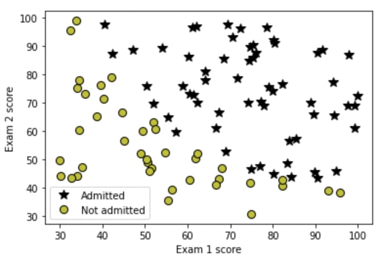
So what we basically want from Logistic Regression is to tell us whether a certain student with some scores of Exam1 and Exam2 is admitted or not. Let's create an instance of the
LogisticRegression class and try it out.Firstly I'm going to find the optimal parameters for this dataset and I'm going to show you two ways of doing it.

Sometimes using gradient descent takes a lot of time so for time-saving, I'll show you how you can easily find the parameters by just using
scipy.optimize.minimize function bypassing the cost function into it.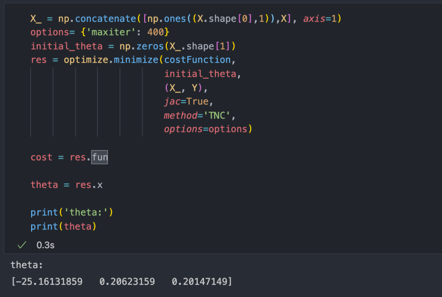
Firstly I appended an extra column of 1s for bias term then pass my
costFunction, initial_theta (initially 0s) and my X and Y as arguments. It easily calculated the optimal parameters in 0.3 seconds much faster than gradient descent which took about 6.5 seconds.Note: costFunction is similar to what we have in our class method as calculate_cost, I just put it outside to show you the work of scipy.optimize.minimize function.
Great now let's see how well it's performed by printing out its accuracy on the training set.
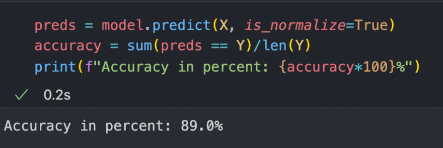
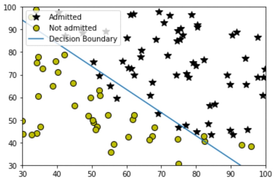
Hmmm, around 89%, it seems good although there are a few algorithms that we'll be covering in future that can perform way much better than this. Now let me show you its decision boundary, as we can see that we didn't perform any polynomial transformation (for more refer to article 2) on our input features so the decision boundary is going to be a straight line.
That's so great we just implemented our
LogisticRegression class on the student's dataset. Let's move ahead and understand the problem of overfitting in the next section. Till then have a short 5-minute break.In order to understand overfitting in Logistic Regression, I'll show you an implementation of this algorithm on another dataset where we need to fit a non-linear decision boundary. Let's visualize our 2nd dataset on the graph:
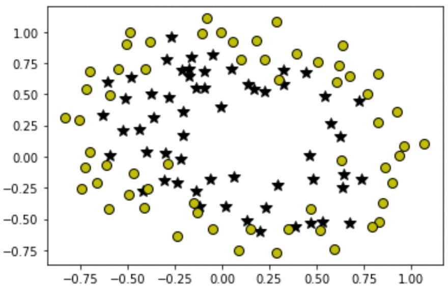
As we can see, it's not linearly separable data so we need to fit a non-linear decision boundary. If you went through the 2nd article of this series then you probably know how we do this, but in brief, we take our original features and apply polynomial transformations on them, like squaring, cubing or multiplying with each other to obtain new features and then training our algorithm on those new features results in non-linear classification.
In the notebook you'll find a function
mapFeature that take individual features as input and return new transformed features. If you wanna know how it's working then consider referring to the notebook and it's recommended to follow it while reading this article.
After getting the new transformed features and following the exact steps we followed in the above section, you'll be able to print out its decision boundary that will look something like this:
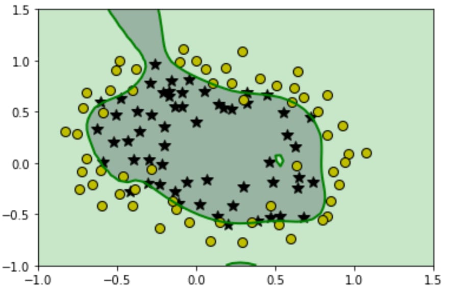
After seeing it, you probably may say that "WOW!, it performed so well almost classified all the training points". Well, it does seem good but in reality, it's worst. Our hypothesis fitted so well on the training set that it loses the generality that means if we provide a new set of points that is not in the training set then our hypothesis will not be able to classify it clearly.
In short, it's necessary to maintain the generality in our hypothesis so that it can perform well on the data it is never seen. Regularization is the way to achieve it. Let's see how to maintain generality using Regularization in the next section.
In this section, we'll be discussing how to implement regularization. Overfitting occurs when the algorithm provides heavy parameters to some features according to the training dataset and hyperparameters. This makes those features dominant in the overall hypothesis and lead to a nice fit in the training set but not so good on the samples outside the training set.
The plan is to add the square of parameters by multiplying them with some big number (λ) to the cost function because our algorithms' main motive is to decrease the cost function, so in this way, the algorithm will end up giving the small parameters just to cancel the effect addition of parameters by multiplying with a large number (λ). So our final cost function gets modified to:

Note: We denote the bias term as θ0 and it's not needed to regularized the bias term that's why we are only considering only θ1 to θn parameters.
Since our cost function is changed that's why our formulas for gradients were also get affected. The new formula for the gradient are:

The new formulas for gradients can be easily derived by partially differentiating the new cost function J(θ) w.r.t to some θj.
Calculating of gradients from cost function is demonstrated in 2nd Article.
λ is known as a regularization parameter and it should be greater than 0. Large value of λ leads to underfitting and very small values lead to overfitting, so you need to pick the right one for your dataset through iterating on some sample values.
We only need to modify the
calculate_cost method because only this method is responsible for calculating both cost and gradients. The modified version is shown below:class RegLogisticRegression:
def __init__(self) -> None:
self.X = None
self.Y = None
self.parameters = None
self.cost_history = []
self.mu = None
self.sigma = None
def sigmoid(self, x):
z = np.array(x)
g = np.zeros(z.shape)
g = 1/(1 + np.exp(-z) )
return g
def sigmoid_derivative(self, x):
derivative = self.sigmoid(x) * (1 - self.sigmoid(x))
return derivative
def calculate_cost(self, lambda_):
"""
Returns the cost and gradients.
parameters: None
Returns:
cost : Caculated loss (scalar).
gradients: array containing the gradients w.r.t each parameter
"""
m = self.X.shape[0]
z = np.dot(self.X, self.parameters)
z = z.reshape(-1)
z = z.astype(np.float128, copy=False)
y_hat = self.sigmoid(z)
cost = -1 * np.mean(self.Y*(np.log(y_hat)) + (1-self.Y)*(np.log(1-y_hat))) + lambda_ * (np.sum(self.parameters[1:]**2))/(2*m)
gradients = np.zeros(self.X.shape[1])
for n in range(len(self.parameters)):
if n == 0:
temp = np.mean((y_hat-self.Y)*self.X[:,n])
else:
temp = np.mean((y_hat-self.Y)*self.X[:,n]) + lambda_*self.parameters[n]/m
gradients[n] = temp
# gradients = np.dot(self.X.T, error)/m
return cost, gradients
def init_parameters(self):
"""
Initialize the parameters as array of 0s
parameters: None
Returns:None
"""
self.parameters = np.zeros((self.X.shape[1],1))
def feature_normalize(self, X):
"""
Normalize the samples.
parameters:
X : input/feature matrix
Returns:
X_norm : Normalized X.
"""
X_norm = X.copy()
mu = np.mean(X, axis=0)
sigma = np.std(X, axis=0)
self.mu = mu
self.sigma = sigma
for n in range(X.shape[1]):
X_norm[:,n] = (X_norm[:,n] - mu[n]) / sigma[n]
return X_norm
def fit(self, x, y, learning_rate=0.01, epochs=500, lambda_=0,is_normalize=True, verbose=0):
"""
Iterates and find the optimal parameters for input dataset
parameters:
x : input/feature matrix
y : target matrix
learning_rate: between 0 and 1 (default is 0.01)
epochs: number of iterations (default is 500)
is_normalize: boolean, for normalizing features (default is True)
verbose: iterations after to print cost
Returns:
parameters : Array of optimal value of weights.
"""
self.X = x
self.Y = y
self.cost_history = []
if self.X.ndim == 1: # adding extra dimension, if X is a 1-D array
self.X = self.X.reshape(-1,1)
is_normalize = False
if is_normalize:
self.X = self.feature_normalize(self.X)
self.X = np.concatenate([np.ones((self.X.shape[0],1)), self.X], axis=1)
self.init_parameters()
for i in range(epochs):
cost, gradients = self.calculate_cost(lambda_=lambda_)
self.cost_history.append(cost)
self.parameters -= learning_rate * gradients.reshape(-1,1)
if verbose:
if not (i % verbose):
print(f"Cost after {i} epochs: {cost}")
return self.parameters
def predict(self,x, is_normalize=True, threshold=0.5):
"""
Returns the predictions after fitting.
parameters:
x : input/feature matrix
Returns:
predictions : Array of predicted target values.
"""
x = np.array(x, dtype=np.float64) # converting list to numpy array
if x.ndim == 1:
x = x.reshape(1,-1)
if is_normalize:
for n in range(x.shape[1]):
x[:,n] = (x[:,n] - self.mu[n]) / self.sigma[n]
x = np.concatenate([np.ones((x.shape[0],1)), x], axis=1)
return [1 if i > threshold else 0 for i in self.sigmoid(np.dot(x,self.parameters))]Now we have our regularized version of
RegLogisticRegression class. Let's address the previous problem of overfitting on polynomial regression by using a set of values for λ to pick the right one.

I can say that λ=1 and λ=10 looks pretty good and they both are able to maintain the generality in hypothesis, the curve is more smooth and less wiggling type. But we can see that as we keep increasing the value if λ the more our hypothesis starts to underfit the data. It basically means that it starts to perform even worst on the training set. Let's visualise the underfitting by plotting cost functions for each λ
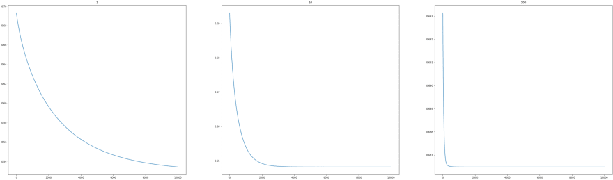
We can see that as λ increases cost also increases. So it's advised to select the value for λ carefully according to your custom dataset.
Great work everyone, we successfully learnt and implemented Logistic Regression. Most people don't write their Machine Learning algorithm from scratch instead they use libraries like Scikit-Learn. Scikit-Learn contains wrappers for many Machine Learning algorithms and it's really flexible and easy to use. But it's not harmful to know about the algorithm you're going to use and the best way of doing it is to understand the underlying mathematics and implement it from scratch.
So in the next article, we'll be making a classification project using the Scikit-Learn library and you'll see how easy it is to use for making some really nice creative projects.
I hope you have learnt something new, for more updates on upcoming articles get connected with me through Twitter and stay tuned for more. Till then enjoy your day and keep learning.
58