
39
Predict which Scooby Doo monsters 👻 are REAL with a tuned decision tree model
This is the latest in my series of screencasts demonstrating how to use the tidymodels packages, from just getting started to tuning more complex models. Today’s screencast walks through how to train and evalute a random forest model, with this week’s
#TidyTuesday dataset on Scooby Doo episodes. 👻Here is the code I used in the video, for those who prefer reading instead of or in addition to video.
Our modeling goal is to predict which Scooby Doo monsters are real and which are not, based on other characteristics of the episode.
library(tidyverse)
scooby_raw <- read_csv("https://raw.githubusercontent.com/rfordatascience/tidytuesday/master/data/2021/2021-07-13/scoobydoo.csv")

scooby_raw %>%
  filter(monster_amount > 0) %>%
  count(monster_real)


## # A tibble: 2 x 2
## monster_real n
## <chr> <int>
## 1 FALSE 404
## 2 TRUE 112
Most monsters are not real!
How did the number of real vs. fake monsters change over the decades?
scooby_raw %>%
  filter(monster_amount > 0) %>%
  count(
    year_aired = 10 * ((lubridate::year(date_aired) + 1) %/% 10),
    monster_real
  ) %>%
  mutate(year_aired = factor(year_aired)) %>%
  ggplot(aes(year_aired, n, fill = monster_real)) +
  geom_col(position = position_dodge(preserve = "single"), alpha = 0.8) +
  labs(x = "Date aired", y = "Monsters per decade", fill = "Real monster?")
How are these different episodes rated on IMDB?
scooby_raw %>%
  filter(monster_amount > 0) %>%
  mutate(imdb = parse_number(imdb)) %>%
  ggplot(aes(imdb, after_stat(density), fill = monster_real)) +
  geom_histogram(position = "identity", alpha = 0.5) +
  labs(x = "IMDB rating", y = "Density", fill = "Real monster?")
It looks like there are some meaningful relationships there that we can use for modeling, but they are not linear so a decision tree may be a good fit.
Let’s start our modeling by setting up our “data budget.” We’re only going to use the year each episode was aired and the episode rating.
library(tidymodels)

set.seed(123)
scooby_split <- scooby_raw %>%
  mutate(
    imdb = parse_number(imdb),
    year_aired = lubridate::year(date_aired)
  ) %>%
  filter(monster_amount > 0, !is.na(imdb)) %>%
  mutate(
    monster_real = case_when(
      monster_real == "FALSE" ~ "fake",
      TRUE ~ "real"
    ),
    monster_real = factor(monster_real)
  ) %>%
  select(year_aired, imdb, monster_real, title) %>%
  initial_split(strata = monster_real)
scooby_train <- training(scooby_split)
scooby_test <- testing(scooby_split)

set.seed(234)
scooby_folds <- bootstraps(scooby_train, strata = monster_real)
scooby_folds


## # Bootstrap sampling using stratification
## # A tibble: 25 x 2
## splits id
## <list> <chr>
## 1 <split [375/133]> Bootstrap01
## 2 <split [375/144]> Bootstrap02
## 3 <split [375/140]> Bootstrap03
## 4 <split [375/132]> Bootstrap04
## 5 <split [375/139]> Bootstrap05
## 6 <split [375/134]> Bootstrap06
## 7 <split [375/146]> Bootstrap07
## 8 <split [375/132]> Bootstrap08
## 9 <split [375/143]> Bootstrap09
## 10 <split [375/143]> Bootstrap10
## # … with 15 more rows
Next, let’s create our decision tree specification. It is tunable, and we could not fit this right away to data because we haven’t said what the model parameters are yet.
tree_spec <-
  decision_tree(
    cost_complexity = tune(),
    tree_depth = tune(),
    min_n = tune()
  ) %>%
  set_mode("classification") %>%
  set_engine("rpart")

tree_spec


## Decision Tree Model Specification (classification)
##
## Main Arguments:
## cost_complexity = tune()
## tree_depth = tune()
## min_n = tune()
##
## Computational engine: rpart
Let’s set up a grid of possible model parameters to try.
tree_grid <- grid_regular(cost_complexity(), tree_depth(), min_n(), levels = 4)
tree_grid


## # A tibble: 64 x 3
## cost_complexity tree_depth min_n
## <dbl> <int> <int>
## 1 0.0000000001 1 2
## 2 0.0000001 1 2
## 3 0.0001 1 2
## 4 0.1 1 2
## 5 0.0000000001 5 2
## 6 0.0000001 5 2
## 7 0.0001 5 2
## 8 0.1 5 2
## 9 0.0000000001 10 2
## 10 0.0000001 10 2
## # … with 54 more rows
Now let’s fit each possible parameter combination to each resample. By putting non-default metrics into
metric_set(), we can specify which metrics are computed for each resample.doParallel::registerDoParallel()
set.seed(345)
tree_rs <-
tune_grid(
tree_spec,
monster_real ~ year_aired + imdb,
resamples = scooby_folds,
grid = tree_grid,
metrics = metric_set(accuracy, roc_auc, sensitivity, specificity)
)
tree_rs
## # Tuning results
## # Bootstrap sampling using stratification
## # A tibble: 25 x 4
## splits id .metrics .notes
## <list> <chr> <list> <list>
## 1 <split [375/133]> Bootstrap01 <tibble [256 × 7]> <tibble [0 × 1]>
## 2 <split [375/144]> Bootstrap02 <tibble [256 × 7]> <tibble [0 × 1]>
## 3 <split [375/140]> Bootstrap03 <tibble [256 × 7]> <tibble [0 × 1]>
## 4 <split [375/132]> Bootstrap04 <tibble [256 × 7]> <tibble [0 × 1]>
## 5 <split [375/139]> Bootstrap05 <tibble [256 × 7]> <tibble [0 × 1]>
## 6 <split [375/134]> Bootstrap06 <tibble [256 × 7]> <tibble [0 × 1]>
## 7 <split [375/146]> Bootstrap07 <tibble [256 × 7]> <tibble [0 × 1]>
## 8 <split [375/132]> Bootstrap08 <tibble [256 × 7]> <tibble [0 × 1]>
## 9 <split [375/143]> Bootstrap09 <tibble [256 × 7]> <tibble [0 × 1]>
## 10 <split [375/143]> Bootstrap10 <tibble [256 × 7]> <tibble [0 × 1]>
## # … with 15 more rowsAll done!
Now that we have tuned our decision tree model, we can choose which set of model parameters we want to use. What are some of the best options?
show_best(tree_rs)


## # A tibble: 5 x 9
## cost_complexity tree_depth min_n .metric .estimator mean n std_err
## <dbl> <int> <int> <chr> <chr> <dbl> <int> <dbl>
## 1 0.0000000001 10 2 accuracy binary 0.872 25 0.00481
## 2 0.0000001 10 2 accuracy binary 0.872 25 0.00481
## 3 0.0001 10 2 accuracy binary 0.872 25 0.00481
## 4 0.0000000001 15 2 accuracy binary 0.871 25 0.00456
## 5 0.0000001 15 2 accuracy binary 0.871 25 0.00456
## # … with 1 more variable: .config <chr>
We can visualize all of the combinations we tried.
autoplot(tree_rs) + theme_light(base_family = "IBMPlexSans")
If we used
select_best(), we would pick the numerically best option. However, we might want to choose a different option that is within some criteria of the best performance, like a simpler model that is within one standard error of the optimal results. We finalize our model just like we finalize a workflow, as shown in previous posts.simpler_tree <- select_by_one_std_err(tree_rs,
-cost_complexity,
metric = "roc_auc"
)
final_tree <- finalize_model(tree_spec, simpler_tree)Now we can fit
final_tree to our training data.final_fit <- fit(final_tree, monster_real ~ year_aired + imdb, scooby_train)We also could use
last_fit() instead of fit(), by swapping out the split for the training data. This will fit one time on the training data and evaluate one time on the testing data.final_rs <- last_fit(final_tree, monster_real ~ year_aired + imdb, scooby_split)This is the first time we have used the testing data through this whole analysis, and let’s us see how our model performs on the testing data. A bit worse, unfortunately!
collect_metrics(final_rs)


## # A tibble: 2 x 4
## .metric .estimator .estimate .config
## <chr> <chr> <dbl> <chr>
## 1 accuracy binary 0.857 Preprocessor1_Model1
## 2 roc_auc binary 0.780 Preprocessor1_Model1
Finally, we can use the parttree package to visualize our decision tree results.
library(parttree)

scooby_train %>%
  ggplot(aes(imdb, year_aired)) +
  geom_parttree(data = final_fit, aes(fill = monster_real), alpha = 0.2) +
  geom_jitter(alpha = 0.7, width = 0.05, height = 0.2, aes(color = monster_real))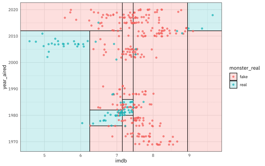
39